
线性回归
先从一个图例来认识线性回归
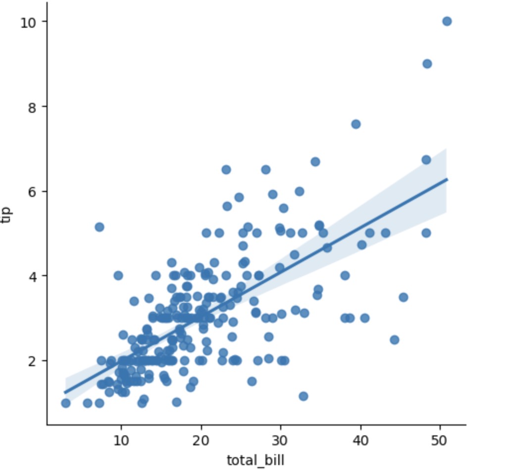
下面用这个公式来实现线性回归 样例数据集
$$\hat{y_i} = \bar{y} + r \frac{SD(y)}{SD(x)} (x_i - \bar{x})$$
1
2
3
4
5
6
| x_bar = np.mean(tips["total_bill"])
y_bar = np.mean(tips["tip"])
std_x = np.std(tips["total_bill"])
std_y = np.std(tips["tip"])
r = np.corrcoef(tips['total_bill'],tips['tip'])[0][1]
r
|
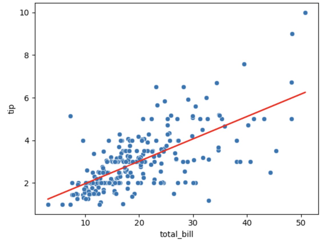
根据上述系数和截距来画图
1
2
3
4
5
| regression = a_hat + b_hat * tips['total_bill']
sns.scatterplot(x="total_bill", y="tip", data=tips)
plt.plot(tips["total_bill"], regression, color="r")
plt.xlabel("total_bill")
plt.ylabel("tip");
|
使用Minimize
L2优化
$$R(a, b) = \frac{1}{n} \sum_{i = 1}^n(y_i - (a + b x_i))^2$$
1
2
3
4
5
6
| def l2_tip_risk_list(theta):
"""Returns average l2 loss between regression line for intercept a
and slope b"""
a = theta[0]
b = theta[1]
return np.mean(np.power(tips['tip']-(a+b*tips['total_bill']),2))
|
多元线性回归
数据集
多元线性回归公式:
$$y_i = \theta_0 + \theta_1 x_1 + \theta_2 x_2 + … + \theta_p x_p $$
1
2
3
4
5
6
7
8
9
|
desired_columns = ['horsepower','hp^2','model_year','acceleration']
model_many = LinearRegression()
model_many.fit(X=vehicle_data[desired_columns], y=vehicle_data["mpg"])
predicted_mpg_many = model_many.predict(
    vehicle_data[["horsepower", "hp^2", "model_year", "acceleration"]]
)
sns.scatterplot(x="horsepower", y="mpg", data=vehicle_data)
plt.plot(vehicle_data["horsepower"], predicted_mpg_many, color="r");
|
